Maximum Likelihood Estimation of Gumbel Distribution

This write up assumes basic knowledge of the estimation theory.

Let’s start with the probability density function of the gumbel distribution, which is

$$p(x)=\frac{1}{\beta}e^{\frac{x-\alpha}{\beta}}e^{-e^{\frac{x-\alpha}{\beta}}}$$

$$\text{where }\alpha \text{ and } \beta \text{ are parameters and }\alpha \in \mathbb{R}, \beta > 0$$

Maximum liklihood solution can be written as,

$$\mathrm{f}_{M L}=\underset{\alpha \in \mathbb{R}, \beta>0}{\operatorname{argmax}} \in \mathbb{R}, \beta>0(P(D | \alpha, \beta))$$

where D represents the set of datapoints.

$$\mathrm{f}{M L}=\underset{\alpha \in \mathbb{R}, \beta>0}{\operatorname{argmax}} \in \mathbb{R}, \beta>0(\prod{i=1}^n P(x_i | \alpha, \beta))$$

where x_i represents each datapoint.

Now onto calculating the log-likelihood,

$$=\ln \left(\prod_{i=0}^{n} P\left(x_{i} | \alpha, \beta\right)\right)$$

$$=\sum_{i=0}^{n} \ln P\left(\left(x_{i} | \alpha, \beta\right)\right)$$

$$=\sum_{i=0}^{n} \ln \left(\frac{1}{\beta} e^{-\frac{y_{i}-\alpha}{\beta}} e^{-e^{-\frac{j_{j}-a}{\beta}}}\right)$$

We end up with an equation with 2 variables in it, we’ll be using the Newton-Raphson method to approximate the roots of the equation. I recommend reading through the link if you’re familiar with the approximation method.

Finding derivatives, with respect to both α and β.

$$\frac{\partial f}{\partial \beta}=\sum_{i=0}^{n} \frac{x_{i}-n}{\beta^{2}}-\frac{n}{\beta}-\sum_{i=0}^{n} \frac{x_{i}-\alpha}{\beta} e^{-\frac{z_{i}-\alpha}{\beta}}$$

$$\frac{\partial f}{\partial \alpha}=\frac{n}{\beta}-\frac{1}{\beta} \sum_{i=0}^{n} e^{-\frac{z_{i}-\alpha}{\beta}}$$

For the Newron-Raphson approximation method, we require double derivatives, which we use to calculate the Hessian matrix.

$$\frac{\partial^{2} f}{\partial \beta^{2}}=\frac{n}{\beta^{2}}-\frac{2}{\beta^{2}} \sum_{i=0}^{n}\left(x_{i}-\alpha\right)+\frac{2}{\beta^{3}} \sum_{i=0}^{n}\left(x_{i}-\alpha\right) e^{\frac{-\left(x_{i}-\alpha\right)}{\beta}}+\frac{2}{\beta^{4}} \sum_{i=0}^{n}\left(x_{i}-\alpha\right)^{2} e^{\frac{-\left(x_{j}-\alpha\right)}{\beta}}$$

$$\frac{\partial^{2} f}{\partial \alpha^{2}}=\frac{-i}{\beta^{2}} \sum_{i=0}^{n} e^{-\frac{x_{i}-a}{\beta}}$$

$$\frac{\partial^{2} f}{\partial \alpha \beta}=-\frac{n}{\beta^{2}}+\frac{1}{\beta^{2}} \sum_{i=0}^{n} e^{\frac{-\left(x_{i}-\alpha\right)}{\beta}}-\frac{1}{\beta^{3}} \sum_{i=0}^{n}\left(x_{i}-\alpha\right) e^{\frac{-\left(x_{i}-a\right)}{\beta}}$$

The Hessian matrix can be calculated by,

$$H=\left[\begin{array}{ll}\frac{\partial^{2} f}{\partial \alpha^{2}} & \frac{\partial^{2} f}{\partial \alpha \beta} \ \frac{\partial^{2} f}{\partial \alpha \beta} & \frac{\partial^{2} f}{\partial \beta^{2}}\end{array}\right]$$

We also need a f matrix with the equations we’re solving for,

$$f=\left[\begin{array}{l}\frac{\partial f}{\partial \alpha} \ \frac{\partial f}{\partial \beta}\end{array}\right]$$

Now we can follow the following algorithm to estimate the parameters.

Step 1 : We’ll choose starting values for α and β, α(0) and β(0) using the method of moment estimators.

β = 0.7977∗ standard deviation of the dataset α = mean of the dataset - 0.4501 * standard deviation

Step 2 :

Choose a tolerance t for the change, 10^(−10) in our case. If the level of changes are less than the tolerance the iterations will break.

Step 3 :

Obtain inverse of the Hessian Matrix inv(H(α(0))(β(0))) and f(α(0))(β(0))

Step 4 :

Obtain new values of α and β, α(new) and β(new), from the Newton Raphson algorithm,

$$\left[\begin{array}{l}\alpha^{(n e w)} \ \beta^{(n e w)}\end{array}\right]=\left[\begin{array}{l}\alpha^{(o l d)} \ \beta^{(o l d)}\end{array}\right]-H^{-1}\left(\alpha^{(o l d)}, \beta^{(o l d)}\right) f\left(\alpha^{(o l d)}, \beta^{(o l d)}\right)$$

Step 5 :

Check to see if the differences between new and the old values are small enough and compare it by the set tolerance,

$$\left[\left(\alpha^{(n e w)}-\alpha^{(o l d)}\right)^{2}+\left(\beta^{(n e w)}-\beta^{(o l d)}\right)^{2}<t\right]$$

• if No, then return to Step(3), and calculate H−1(α(new))(β(new)) and f(α(new))(β(new)) and keep iterating.
• if Yes, then stop.

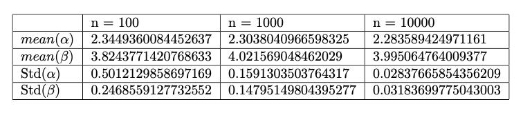
Following are the results of the above algorithm for a gumbel destibution generated using α = 2.3 and β = 4.0 ran multiple times and averaged.

Link to the code.